Flowchart

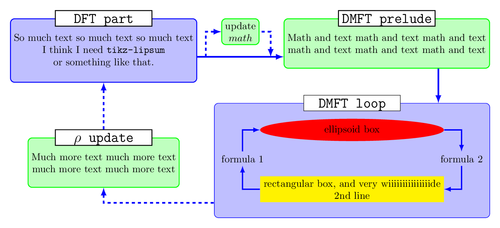
This example flowchart uses the positioning-plus library and the node-families library by the same author. The fit library is implicitly loaded by positioning-plus, the backgrounds library is used to draw stuff behind other stuff, the calc library for some coordinate calculations and the shapes.geometric library for the ellipse shape.

This example was written by Qrrbrbirlbel answering a question on TeX.SE.

Edit and compile if you like:

% Flowchart
% Author: Qrrbrbirlbel
\documentclass[tikz,border=10pt]{standalone}
\usetikzlibrary{shapes.geometric,backgrounds,
  positioning-plus,node-families,calc}
\tikzset{
  basic box/.style = {
    shape = rectangle,
    align = center,
    draw  = #1,
    fill  = #1!25,
    rounded corners},
  header node/.style = {
    Minimum Width = header nodes,
    font          = \strut\Large\ttfamily,
    text depth    = +0pt,
    fill          = white,
    draw},
  header/.style = {%
    inner ysep = +1.5em,
    append after command = {
      \pgfextra{\let\TikZlastnode\tikzlastnode}
      node [header node] (header-\TikZlastnode) at (\TikZlastnode.north) {#1}
      node [span = (\TikZlastnode)(header-\TikZlastnode)]
        at (fit bounding box) (h-\TikZlastnode) {}
    }
  },
  hv/.style = {to path = {-|(\tikztotarget)\tikztonodes}},
  vh/.style = {to path = {|-(\tikztotarget)\tikztonodes}},
  fat blue line/.style = {ultra thick, blue}
}
\begin{document}
\begin{tikzpicture}[node distance = 1.2cm, thick, nodes = {align = center},
    >=latex]
  \node[Minimum Width = loop, shape = ellipse, fill = red] (imp-sol)
    {ellipsoid box};
  \node[Minimum Width = loop, fill = yellow, below = of imp-sol] (rec-box)
    {rectangular box, and very wiiiiiiiiiiiiiiide\\2nd line};
  \node[shift = (left:.5*x_node_dist)] at
    ($(imp-sol.west|-imp-sol.south)!.5!(rec-box.north west)$) (for-1)
    {formula 1};
  \node[shift = (right:.5*x_node_dist)] at
    ($(imp-sol.east|-imp-sol.south)!.5!(rec-box.north east)$) (for-2)
    {formula 2};
  \begin{scope}[on background layer]
    \node[fit = (for-1)(for-2)(imp-sol)(rec-box), basic box = blue,
      header = DMFT loop] (dmft-l) {};
  \end{scope}
  \path[very thick, blue, hv] (rec-box) edge[->] (for-1) edge[<-] (for-2)
                              (imp-sol) edge[->] (for-2) edge[<-] (for-1);

  \node[east above = of dmft-l, basic box = green, header = DMFT prelude]
    (dmft-p) {Math and text math and text math and text\\
              math and text math and text math and text};
  \node[north left = of dmft-l, basic box = green, header = $\rho$ update,
     shift = (down:y_node_dist)] (rho)
    {Much more text much more text\\much more text much more text};
  \node[basic box = blue, header = DFT part, anchor = north] at
    (dmft-p.north-|rho) (dft) {So much text so much text so much text\\
    I think I need \texttt{tikz-lipsum}\\or something like that.};
  \node[basic box = green, anchor = north] at
    ($(dft.north east)!.5!(dmft-p.north west)$) (upd) {update\\$math$};
  \path[fat blue line, <-, dashed, vh] (rho) edge
    ({$(rho.south)!.5!(dmft-l.south)$}-|dmft-l.south west);
  \path[fat blue line, ->]
    ({$(upd.south)!.5!(dmft-p.south)$}-|dmft-p.south west)
    coordinate (@) edge[<-, solid] coordinate[pos=.15] (@s)
    coordinate[pos=.9] (@e) (@-|dft.east)
    {[every edge/.append style=dashed, vh] (@s) edge[<-] (upd) (@e) edge (upd)}
    (h-rho) edge[dashed] (dft)
    ($(dmft-p.south)!.5!(dmft-p.south east)$)
    coordinate (@) edge (@|-dmft-l.north);
\end{tikzpicture}
\end{document}