Control system principles

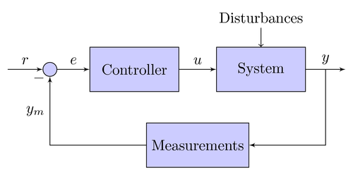
An example of a control system with a feedback loop. Block diagrams like this are quite time consuming to create by hand. The relative node placement feature makes it a bit easier, but it works best when the nodes have equal widths. However, the results are quite pleasing and hopefully worth the effort. You can probably speed up the process by creating custom macros.

Edit and compile if you like:

\documentclass{article}

\usepackage{tikz}
\usetikzlibrary{shapes,arrows}


\begin{document}


\tikzstyle{block} = [draw, fill=blue!20, rectangle, 
    minimum height=3em, minimum width=6em]
\tikzstyle{sum} = [draw, fill=blue!20, circle, node distance=1cm]
\tikzstyle{input} = [coordinate]
\tikzstyle{output} = [coordinate]
\tikzstyle{pinstyle} = [pin edge={to-,thin,black}]

% The block diagram code is probably more verbose than necessary
\begin{tikzpicture}[auto, node distance=2cm,>=latex']
    % We start by placing the blocks
    \node [input, name=input] {};
    \node [sum, right of=input] (sum) {};
    \node [block, right of=sum] (controller) {Controller};
    \node [block, right of=controller, pin={[pinstyle]above:Disturbances},
            node distance=3cm] (system) {System};
    % We draw an edge between the controller and system block to 
    % calculate the coordinate u. We need it to place the measurement block. 
    \draw [->] (controller) -- node[name=u] {$u$} (system);
    \node [output, right of=system] (output) {};
    \node [block, below of=u] (measurements) {Measurements};

    % Once the nodes are placed, connecting them is easy. 
    \draw [draw,->] (input) -- node {$r$} (sum);
    \draw [->] (sum) -- node {$e$} (controller);
    \draw [->] (system) -- node [name=y] {$y$}(output);
    \draw [->] (y) |- (measurements);
    \draw [->] (measurements) -| node[pos=0.99] {$-$} 
        node [near end] {$y_m$} (sum);
\end{tikzpicture}

\end{document}